Cycloid
The cycloid is traced out by a point on a wheel which is rolling, without slipping, along a flat horizontal surface. The maximum height of the curve is therefore the diameter of the wheel.
The cycloid can be plotted using the following parametric equations. The equation for y shows that the 'r' parameter in the equations is the radius of the wheel.
\begin{align*} x &= r (t - sin(t)) \\ y &= r (1 - cos(t)) \end{align*}This can be plotted using the Julia 'Plots' library as follows:
            using Plots
            r = 0.1
            t = range(0, 4 * pi, length=400)
            x = r * (t .- sin.(t))
            y = r * (1 .- cos.(t))
            p = plot(x, y, aspect_ratio = :equal, framestyle = :origin, legend = false, size = (500, 200))
            ylims!(0, 0.3)
            title!("Cycloid")
            xlabel!("x")
            ylabel!("y")
            png(p, "cycloid")
            gui(p)
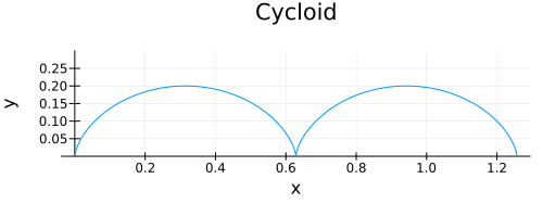
The output is:

From a Julia coding point of view one item of interest is that the combination of broadcasting the minus sign in the equations and broadcasting the sin and cos functions works just as you would hope: the x and y values are the ranges needed to plot the cycloid. This completely avoids any form of explicit loops.
By default the plot is scaled so that it is approximately square. This makes the cycloid look taller than it should. To stretch it out to the correct proportions we use the aspect_ratio keyword.
To make the axes intesect at the origin we use the framestyle keyword.
To specify that labels, e.g. for the y variable, are not required we use the legend keyword.
To specify the size of the image we supply size = (width, height).
We can modify the current plot to limit the values displayed on the y axis, to provide a title and labels for the axes.
The code can be run in the REPL. It saves the output to a png file called 'cycloid.png' in the current directory. It also shows the graph in a graphic window on the screen.
It might be interesting to somehow show the values of the t parameter?
The reason I got interested in the cycloid is that, upside down, it is the curve of fastest descent. There is a fascinating history behind this problem. It leads, ultimately, to the Euler - Lagrange equations which can be used in so many areas of maths and science.
I was thinking about a diagram that had more graphic elements than just the cycloid. In the Plots documentation I came across the following code to do just that.
                using Plots; gr()
                x = range(0, 10, length=100)
                y1 = sin.(x)
                y2 = cos.(x)
                p = plot(x, [y1 y2])
                y3 = @. sin(x)^2 - 1/2
                plot!(p, x, y3)
                png(p, "sin_cos_etc")
                gui(p)
The syntax @. was unfamiliar to me. Its purpose is to dot each function in the expression which follows. This means that the expresssion automatically handles the situation where more than one dot is needed. I wondered if I could have used this in my cycloid code so amended the code as shown below:
                using Plots
                r = 0.1
                t = range(0, 4 * pi, length=400)
                x = @. r * (t - sin(t))
                y = @. r * (1 - cos(t))
                p = plot(x, y, aspect_ratio = :equal, framestyle = :origin, legend = false)
                png(p, "cycloid")
                gui(p)
This turns out to work just fine and is in some ways even more like the math syntax.
The other thing shown in the piece of code is the use of plot! to change an existing plot by adding another element to it. The following draws a circle:
                using Plots
                r = 0.1
                t = range(0, 2 * pi, length=400)
                x = @. r * sin(t)
                y = @. r * cos(t)
                p = plot(x, y, aspect_ratio = :equal, framestyle = :origin, legend = false)
                png(p, "circle")
                gui(p)
If I wanted to draw a plot with multiple graphic objects I would prefer to build up the components in separate functions. A first attempt at combining the cycloid and circle code:
                using Plots

                # Returns a new plot
                function cycloid()
                    r = 0.1
                    t = range(0, 4 * pi, length=400)
                    x = r * (t .- sin.(t))
                    y = r * (1 .- cos.(t))
                    p = plot(x, y, aspect_ratio = :equal, framestyle = :origin, legend = false, size = (500, 200))
                    ylims!(0, 0.3)
                    title!("Cycloid")
                    xlabel!("x")
                    ylabel!("y")
                end

                # Modifies an existing plot by drawing a circle sat on the x-axis at the specified x-offset
                function circle!(p, offset)
                    r = 0.1
                    t = range(0, 2 * pi, length=400)
                    x = @. r * (offset + sin(t))
                    y = @. r * (1 + cos(t))
                    plot!(p, x, y, c=:darkblue)
                end

                # Join pipeline together
                p = cycloid()
                circle!(p, 0)
                circle!(p, pi)
                circle!(p, 2*pi)
                circle!(p, 3*pi)
                circle!(p, 4*pi)

                png(p, "cycloid_and_circles")
                gui(p)
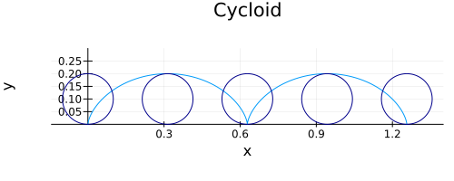
Here is the image:

A slightly neater way of assembling the image is:
            # Join pipeline together
            xPositions = [x * pi for x in 0:4]
            p = cycloid()
            (xpos -> circle!(p, xpos)).(xPositions)

            png(p, "cycloid_and_circles")
            gui(p)
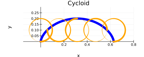
We can also introduce using linewidths to show the circle is rolling along:
            using Plots

            # Returns a new plot
            function cycloid()
                r = 0.1
                t = range(0, 2 * pi, length=200)
                x = r * (t .- sin.(t))
                y = r * (1 .- cos.(t))
                p = plot(x, y, aspect_ratio=:equal, framestyle=:origin, legend=false, linewidth=8, color=:blue, size=(500, 200))
                ylims!(-0.05, 0.3)
                xlims!(-0.15, 0.8)
                title!("Cycloid")
                xlabel!("x")
                ylabel!("y")
                return p
            end

            # Modifies an existing plot by drawing a circle sat on the x-axis at the specified x-offset
            function circle!(p, offset, turn)
                r = 0.1
                len = 100
                t = range(0, 2 * pi, length=len)
                lws = range(0, 6, len)
                x = @. r * (offset + sin(t))
                y = @. r * (1 + cos(t))
                plot!(p, x, y, ; linewidth = circshift(lws, turn),color=:orange)
            end

            # This is the neat way to join components together using broadcasting.
            xPositions = [x * pi for x in 0:0.5:2]
            turns = [50, 75, 0, 25, 50]
            p = cycloid()
            ((xpos, turn) -> circle!(p, xpos, turn)).(xPositions, turns)
            png(p, "images/cycloid_rolling_circle")
            gui(p)
