Plot Recipe

User Recipe

A feature of the Plot library is the use of a recipe. This is an example from the documentation.

            mutable struct MyType end

            @recipe function f(::MyType, n::Integer = 10; add_marker = false)
                linecolor   --> :blue
                seriestype  :=  :path
                markershape --> (add_marker ? :circle : :none)
                delete!(plotattributes, :add_marker)
                rand(n)
            end
            

The arrow --> will set the attribute if it isn't already set. The notation := will force the attribute to have the specified value.

This is how it is used:

            mt = MyType()
            plot(
                plot(mt),
                plot(mt, 100, linecolor = :red),
                plot(mt, marker = (:star,20), add_marker = false),
                plot(mt, add_marker = true)
            )                
            

So, I am wondering if I can adapt this in some way. e.g. could there be a recipe to draw circles? Let's start with the bare code for drawng a circle....

                using Plots
                r = 0.1
                t = range(0, 2 * pi, length=400)
                x = @. r * sin(t)
                y = @. r * cos(t)
                p = plot(x, y, aspect_ratio = :equal, framestyle = :origin, legend = false)
                png(p, "circle")
                gui(p)                
            

And do the bare minimum to turn it into a circle.:

            @recipe function f(::MyType)
                r = 0.1
                t = range(0, 2 * pi, length=400)
                x = @. r * sin(t)
                y = @. r * cos(t)
                [x,y]
            end
            #= Usage:
            mt = MyType()
            plot(mt)
            =#
            

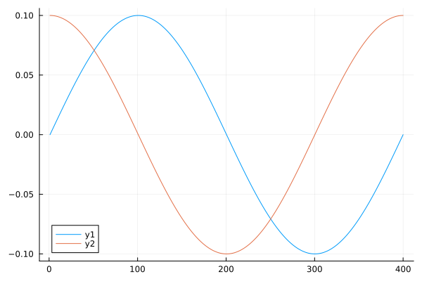
My first effort, above, plots the x and y graphs against t:

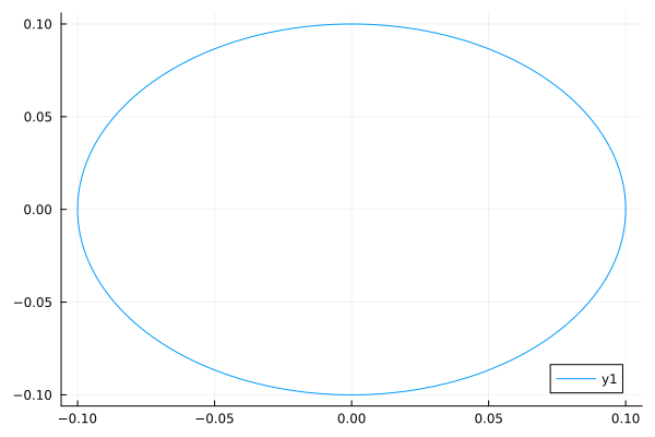
So a guess about how to return the values to be plotted does, sort of, work:

            @recipe function f(::MyType)
                r = 0.1
                t = range(0, 2 * pi, length=400)
                x = @. r * sin(t)
                y = @. r * cos(t)
                (x,y)
            end
            #= Usage:
            mt = MyType()
            plot(mt)
            =#
            

So the next step is to put back the attributes which were necessary in the original circle code. aspect_ratio = :equal, framestyle = :origin, legend = false

                @recipe function f(::MyType)
                    aspect_ratio := :equal
                    framestyle := :origin
                    legend := false
                    r = 0.1
                    t = range(0, 2 * pi, length=400)
                    x = @. r * sin(t)
                    y = @. r * cos(t)
                    (x,y)
                end
                #= Usage:
                mt = MyType()
                plot(mt)
                =#
            

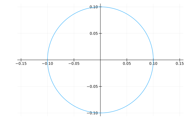
This succeeds in drawing a circle:

Improvements

So, obvious improvements are: to rename the type and allow the radius of the circle to be specified.

            using Plots

            mutable struct Circle end

            @recipe function f(::Circle, radius::Float64 = 1.0)
                aspect_ratio := :equal
                framestyle := :origin
                legend := false
                t = range(0, 2 * pi, length=400)
                x = @. radius * sin(t)
                y = @. radius * cos(t)
                (x,y)
            end

            c = Circle()
            plot(c, 2.0)    # Plot circle of radius 2.0
            plot(c)         # Plot circle with default radius of 1.0
        

Varying line width

The above code draws a circle with a default colour and linewidth. These things can still be specified in the call to the plot function. The next example shows how to vary the linewidth:

        lws = range(0, 10, 400)
        p = plot(c, 1.0; linewidth = lws)
        png(p, "pr1" )
        

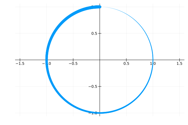
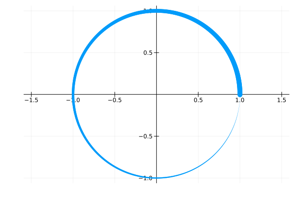
We are approaching the possibility of an animation! Call the image above pr0, meaning rotation of 0 in the linewidths. Produce 3 more images using circshift(lws, 100), then 200 then 300. Call the images pr1, pr2, pr3. The images look like this:

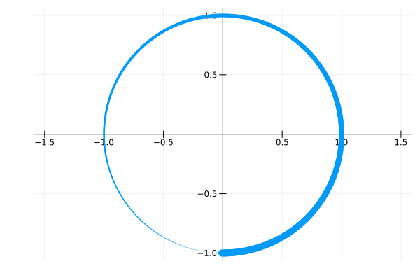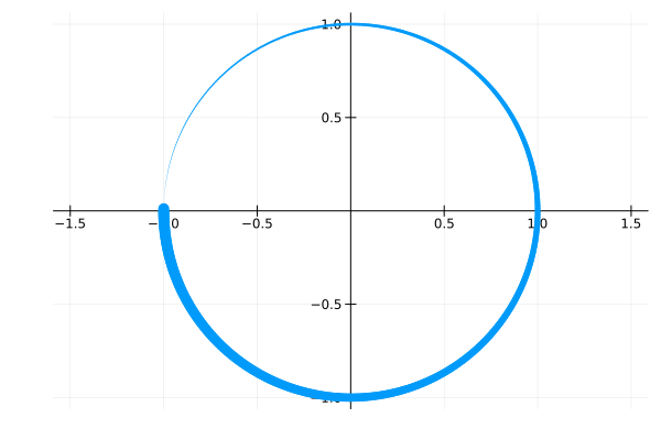Using these images in the order pr2, pr3, pr0, pr1 would work for the cycloid on this page: Cycloid and would match up with the positions shown on that page. The varying linewidth would indicate the direction and amount of rotation.

Step 1 is to automate the production of the png files.

        c = Circle()
        lws = range(0, 10, 400)
        shifts = 0:20:400
        for e in shifts
            p = plot(c, 1.0; linewidth = circshift(lws, e))
            png(p, "pr$(string(e, pad=3))" )
        end
        

The png files can then be turned into an acceptable animation using the following command line:

        convert -delay 10 -loop 5 pr*.png circle.gif
        

I used this to produce a gif which worked but have commented out the display of it. This is because there is an issue with using gifs for animation. There is no simple straightforward way to control when they start, pause, continue or stop. Converting to video would work better and is simple to do:

        convert -delay 10 -loop 5 pr*.png circle.mp4    
        

However, the loop command seems to have been ignored....